Part 3
NHL 19 THREES Data Deep Dive
Analyzing game development using data science
By Brian Maresso & Sean Finlon

Recap
We’re now in Part 3 of our NHL 19 THREES Data Deep Dive- so go back and check out Part 1 and Part 2 to catch up. In Parts 1 and 2, we discussed the distribution of Money Pucks as a Markov Chain, the importance of the +/- stat and its effect on the outcome of games (for better or worse), and the millions of different potential game states that exist in THREES.
In Part 2, we used a brute-force method to generate probability tables for games of given lengths (in pucks). We ran the brute-force method for up to 10-puck length games with the resulting probability table:
| +/- | Chance to Win | Chance to Lose | Chance to Tie |
|---|---|---|---|
| +10 | 100.00000% | 0.00000% | 0.00000% |
| +8 | 100.00000% | 0.00000% | 0.00000% |
| +6 | 99.99901% | 0.00000% | 0.00098% |
| +4 | 99.07636% | 0.22742% | 0.69622% |
| +2 | 81.17651% | 8.68209% | 10.14140% |
| +0 | 40.13809% | 40.13809% | 19.72382% |
| -2 | 8.68209% | 81.17651% | 10.14140% |
| -4 | 0.22742% | 99.07636% | 0.69622% |
| -6 | 0.00000% | 99.99901% | 0.00098% |
| -8 | 0.00000% | 100.00000% | 0.00000% |
| -10 | 0.00000% | 100.00000% | 0.00000% |
The alternative way of viewing the probability table can be found here. In this document, each row represents the number of pucks scored in the game and each column represents the +/- of one team. The resulting values tell us the probability that this team won the game given the game length and +/-.
Introduction
The methodology in Part 2 for finding probability tables was solid, but did not scale well. Our data from Part 1 tells us that our average game length is about 14.8 pucks (Note that THREES shows the value of the current puck in addition to the upcoming three pucks, so the last three pucks recorded are never actually scored. We reduce the recorded puck count by 3 when computing the average to account for this). Since the brute-force method could only go up to 10-puck games, it was not applicable to actual games which typically run longer. Future work might include optimization of the brute-force method- which could provide precise probability tables higher than 10.
Instead, we will focus this section on deriving an approximation function which outputs probability to win based on game length and +/-. Using this function will let us calculate the expected probability to win games of more realistic lengths. This will allow us to answer the question for this article:
The Big Question:
How can we approximate the probability that a team will win a THREES game of any length?
Section 1: Early Observations
During our research into Part 2, we noticed that when the we plotted win probability along the y-axis when +/- was on the x-axis, a familiar shape appeared:
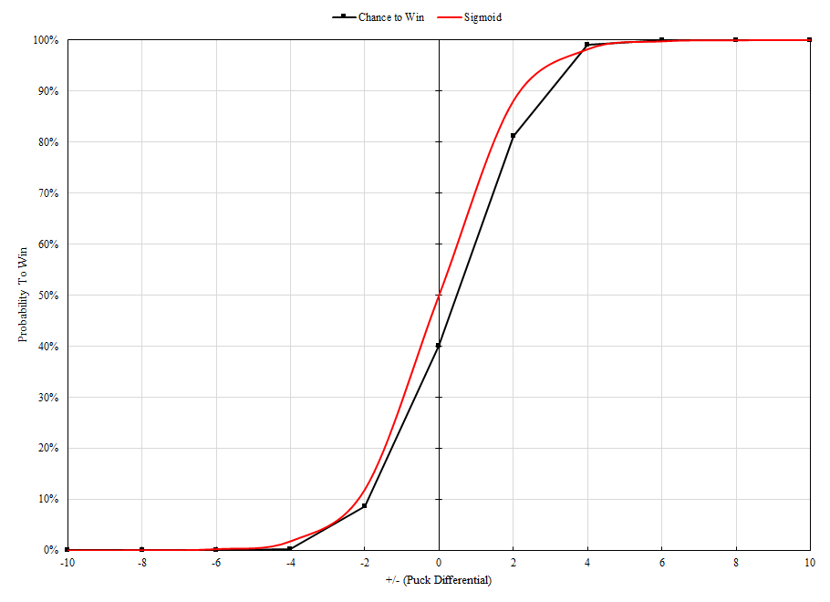
We could see immediately that the general shape of the ‘Chance to Win’ plot was very similar to the Sigmoid function, the most basic form the the logistic function (shown in red). Logistic functions are most notably used in the ecology world as a model for population growth of species. They can also be used in the statistics world, since they resemble the cumulative distribution function (CDF) formed from a standard normal distribution probability density function (PDF), but are still relatively easy to work with. This doesn’t apply in our case, as our model does not represent a CDF, but it is a pretty good model for our win probability. The approximation is decent as-is, but there are discrepancies which invalidate this method for full-scale use. For example, the y-intercept of the Sigmoid function is 0.5 or 50%. Recall from Part 2 that as the number of pucks scored goes to infinity, the probability of a win where +/- is 0 approaches 0.4 or 40%.
With this information in mind, we can begin to consider how to extrapolate an approximation function which scales to our data. The following table is a list all of the factors which we believe influences win probability:
| Variable | Description |
|---|---|
| T | The team we want to find the win probability for |
| G | The total number of pucks which have been scored in this game |
| p | The puck differential (+/-) for T |
| Value | Description |
| W | Represents the winning team |
| P(W=T) | The probability that T wins the game |
Our final approximation function should answer the following:
![]()
Section 2: Curve Fitting
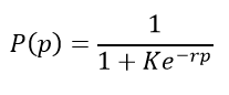
The challenging part of this model is the fact that there are two variables in the desired function- G and p. Our methodology was the use a logistic formula as a function of +/- (p) and fit a formula where the error was minimized for each number of pucks:
Next, we need to use two more formulas to represent the values of K and r. These will be functions of the total number of pucks scored (G). In order to calculate these values, we can compare against the data we retrieved from the brute-force method (assuming our collected data is accurate to long-term trends, then the brute-force data can be considered to be the ground truth).
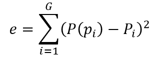
To do this, we tested K and r separately over values in the range [1,10] then calculate the minimum squared error for each combination (see the formula below). In this test, Pi is the probability value corresponding to the observed case at the given +/- and P(Pi) is the model probability value.
The combination of K and r where the error e is minimized would be the “magic numbers” used in the future for corresponding number of pucks. For example, when G=10, the following function was the result of the lowest error value found when K=1.516 and r=0.973:
![]()
This equation produces the following graph:
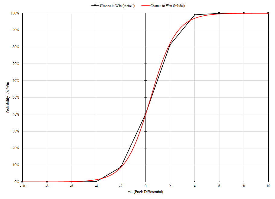
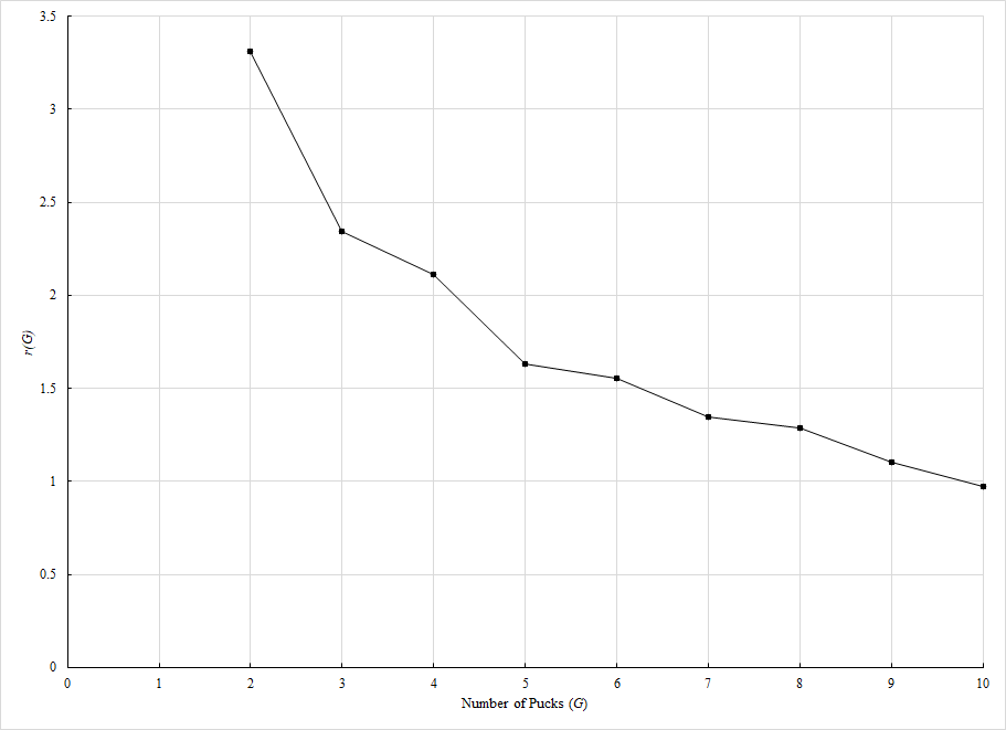
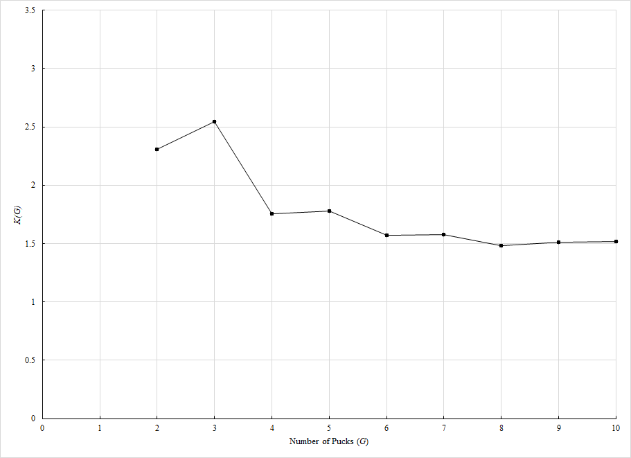
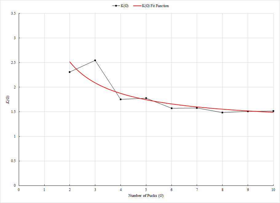
This is a clear improvement over the basic Sigmoid function in terms of approximation accuracy. The given model fits much closer to the ground truth data with significantly lower error. This process is repeated for values of G over the range [1,9] to compare with the rest of our ground truth probability tables. The minimum-error values of the r and K functions for the given number of pucks G can be seen below:
| G | r(G) | K(G) |
| 1 | N/A | N/A |
| 2 | 3.310 | 2.310 |
| 3 | 2.343 | 2.544 |
| 4 | 2.112 | 1.754 |
| 5 | 1.634 | 1.780 |
| 6 | 1.556 | 1.574 |
| 7 | 1.349 | 1.579 |
| 8 | 1.287 | 1.485 |
| 9 | 1.104 | 1.510 |
| 10 | 0.973 | 1.516 |
Note the special case where the number of pucks scored G=1. Regardless of the puck value, the team which scores the one goal will be the winner 100% of the time (in fact- this is the only value of G in THREES where the team which outscored the opponent will always be guaranteed a win). The probability must be 1 when p=1 and 0 when p=0. This pattern can be achieved using the logistic function, but only when r approaches infinity:
![]()
Since e-(1)(∞)=0 and e-(-1)(∞)=∞, then:
![]()
Therefore, P(-1)=0 and P(1)=1/(1+0)=1, which is exactly the relationship we need for G=1. A direct consequence of r being infinite is that we are no longer concerned with the value of K*. The two takeaways from this special case are as follows:
- There is a vertical asymptote at G=1 for the r best-fit function
- When considering the best-fit function, we can ignore K when G=1
*The exception is when K=∞, but we will ignore this theoretical case for now to focus on practical values
Section 3: Probability to Win Approximation
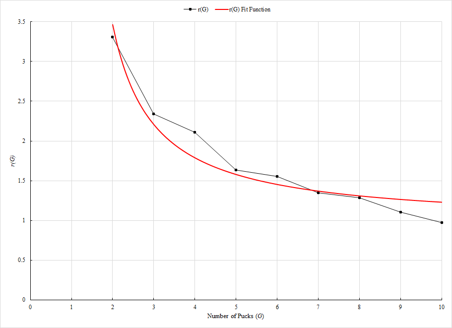
Using our findings from the previous section, we can now calculate the necessary constants to provide a generalized win probability function. First, we must produce a vertical asymptote for r. We do this by creating a fraction with a denominator of G-1. To keep this function as simple as possible, we only used two parameters a and b as fitting variables. More terms could be added to the fit function, but we are in a delicate situation having only 10 data points for our ground truth. When dealing with so few data points, we are at risk of overfitting. The r function will follow the given formula:
![]()
The same method used in the previous section was used to minimize error over our given dataset, and the final r fit function was found to be the following:
![]()
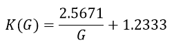
The process for K will be similar to r but the denominator will not have the -1. We know that there cannot be a vertical asymptote at G=1 for K, so we declare new variables c and d for fitting purposes. The K function will follow the given formula:
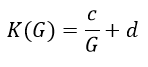
Repeating the process used for r to obtain minimum-error values of c and d, we find the following as the final K function:
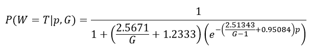
With the final functions for r and K, we can create a single function to accurately model the win W probability for any total number of pucks G and goal differential (+/-) p for the given team T (thus answering our original question):
Section 4: Analysis
It is important to test any model against known data to prove its accuracy. Since our brute-force method cannot calculate games beyond 10 pucks in length, we will test our model against all possible +/- values for games of a length over the range [1,10] and compare the results for each combination. If our model is accurate over this range, then we can apply it to games where more than 10 pucks are scored. Recall from earlier that an average game of THREES is around 14 pucks long**, so the ability to predict win probability for games beyond G=10 is a huge step forward.
The following tables contain every combination of +/- for every game whose puck length is within the range [1,10] (similar to the probability tables seen in Part 2). For each instance, we include the ground truth (found in Part 2 via brute-force) along with the model prediction and the error. The last row contains the average error for the given value of G.
**This figure is collected from our 100-game data spreadsheet seen in Part 1. Note that this data was collected solely from our online ranked matches, which in turn skews the game puck length towards our personal tendencies. While the Money Puck distribution patterns are consistent across all players worldwide, players of varying skill level might see a difference in their average game length. Even so, we believe it is safe to assume that most NHL 19 THREES games will exceed 10 pucks scored on average regardless of player skill level.
G=1
| +/- | Chance to Win (Actual) | Chance to Win (Model) | Error |
|---|---|---|---|
| +1 | 1 | 1 | 0 |
| -1 | 0 | 0 | 0 |
| Mean | 0 |
G=2
| +/- | Chance to Win (Actual) | Chance to Win (Model) | Error |
|---|---|---|---|
| +2 | 1 | 0.997541 | 0.002459 |
| +0 | 0.302082 | 0.284345 | 0.017737 |
| -2 | 0 | 0.000389 | 0.000389 |
| Mean | 0.006862 |
G=3
| +/- | Chance to Win (Actual) | Chance to Win (Model) | Error |
|---|---|---|---|
| +3 | 1 | 0.99723 | 0.00277 |
| +1 | 0.803603 | 0.81319 | 0.009587 |
| -1 | 0.036518 | 0.050009 | 0.013491 |
| -3 | 0 | 0.000636 | 0.000636 |
| Mean | 0.006621 |
G=4
| +/- | Chance to Win (Actual) | Chance to Win (Model) | Error |
|---|---|---|---|
| +4 | 1 | 0.998537 | 0.001463 |
| +2 | 0.972879 | 0.9502 | 0.022679 |
| 0 | 0.36354 | 0.347817 | 0.015723 |
| -2 | 0.002138 | 0.014688 | 0.01255 |
| -4 | 0 | 0.000416 | 0.000416 |
| Mean | 0.010566 |
G=5
| +/- | Chance to Win (Actual) | Chance to Win (Model) | Error |
|---|---|---|---|
| +5 | 1 | 0.99935 | 0.00065 |
| +3 | 0.997751 | 0.98493 | 0.012821 |
| +1 | 0.740663 | 0.735256 | 0.005406 |
| -1 | 0.100784 | 0.105558 | 0.004774 |
| -3 | 0 | 0.00499 | 0.00499 |
| -5 | 0 | 0.000213 | 0.000213 |
| Mean | 0.004809 |
G=6
| +/- | Chance to Win (Actual) | Chance to Win (Model) | Error |
|---|---|---|---|
| +6 | 1 | 0.999729 | 0.000271 |
| +4 | 1 | 0.995066 | 0.004934 |
| +2 | 0.93054 | 0.916792 | 0.013747 |
| 0 | 0.390384 | 0.375777 | 0.014607 |
| -2 | 0.019115 | 0.031843 | 0.012728 |
| -4 | 0 | 0.001794 | 0.001794 |
| -6 | 0 | 9.82E-05 | 9.82E-05 |
| Mean | 0.006993 |
G=7
| +/- | Chance to Win (Actual) | Chance to Win (Model) | Error |
|---|---|---|---|
| +7 | 1 | 0.99989 | 0.00011 |
| +5 | 1 | 0.998306 | 0.001694 |
| +3 | 0.986782 | 0.9744 | 0.012383 |
| +1 | 0.705298 | 0.710893 | 0.005595 |
| -1 | 0.145667 | 0.137079 | 0.008588 |
| -3 | 0.002611 | 0.010158 | 0.007547 |
| -5 | 0 | 0.000663 | 0.000663 |
| -7 | 0 | 4.28E-05 | 4.28E-05 |
| Mean | 0.004578 |
G=8
| +/- | Chance to Win (Actual) | Chance to Win (Model) | Error |
|---|---|---|---|
| +8 | 1 | 0.999956 | 4.37E-05 |
| +6 | 1 | 0.9994 | 0.0006 |
| +4 | 0.998177 | 0.991827 | 0.006351 |
| +2 | 0.893066 | 0.898334 | 0.005268 |
| 0 | 0.405649 | 0.391514 | 0.014135 |
| -2 | 0.041521 | 0.044755 | 0.003234 |
| -4 | 0.000239 | 0.0034 | 0.003161 |
| -6 | 0 | 0.000248 | 0.000248 |
| -8 | 0 | 1.81E-05 | 1.81E-05 |
| Mean | 0.003673 |
G=9
| +/- | Chance to Win (Actual) | Chance to Win (Model) | Error |
|---|---|---|---|
| +9 | 1 | 0.999983 | 1.73E-05 |
| +7 | 1 | 0.999783 | 0.000217 |
| +5 | 0.999822 | 0.997288 | 0.002534 |
| +3 | 0.967315 | 0.966988 | 0.000327 |
| +1 | 0.655636 | 0.699995 | 0.044359 |
| -1 | 0.191471 | 0.15673 | 0.034742 |
| -3 | 0.010123 | 0.014589 | 0.004466 |
| -5 | 1.07E-05 | 0.001178 | 0.001167 |
| -7 | 0 | 9.39E-05 | 9.39E-05 |
| -9 | 0 | 7.48E-06 | 7.48E-06 |
| Mean | 0.008793 |
G=10
| +/- | Chance to Win (Actual) | Chance to Win (Model) | Error |
|---|---|---|---|
| +10 | 1 | 0.999993 | 6.77464E-06 |
| +8 | 1 | 0.999921 | 7.93076E-05 |
| +6 | 0.99999 | 0.999072 | 0.000917797 |
| +4 | 0.990764 | 0.989246 | 0.001517686 |
| +2 | 0.811765 | 0.887098 | 0.07533309 |
| 0 | 0.401381 | 0.401605 | 0.000223913 |
| -2 | 0.086821 | 0.054218 | 0.032603089 |
| -4 | 0.002274 | 0.004873 | 0.002598498 |
| -6 | 0 | 0.000418 | 0.00041807 |
| -8 | 0 | 3.57E-05 | 3.57236E-05 |
| -10 | 0 | 3.05E-06 | 3.05147E-06 |
| Mean | 0.010339727 |
We see that the model is fairly accurate in all instances, rarely exceeding average error marks of over 1%. While there is more optimization to be done, we can consider the model to be reliable for now. To answer our original question ‘How can we approximate the probability that a team will win a THREES game of any length?’: by using the approximation function at the end of Section 3, we can obtain a presumably reliable probability to win given the total number of goals scored G and the given team’s +/- p. For example, our average THREES game contains a total of 14 pucks scored between both teams. Using our approximation function, we obtain the following graph:
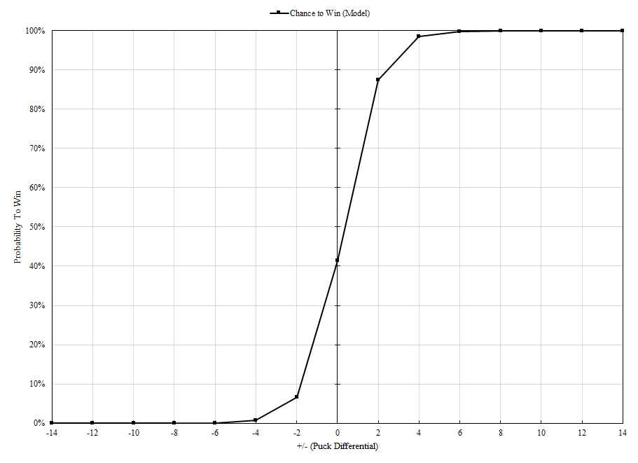
Notice that this graph created using the model maintains the familiar curve we see with our brute-force algorithm. The trend continues to approach its horizontal tangent (either positive or negative) as more unbalanced goals are scored. While we are currently unable to verify data beyond G=10, long-term probability forecasting remains stable even at high values. At this point, one might question why we compare our model to what is essentially another model for verification. To prove the accuracy of our model(s), shouldn’t we be comparing them to actual win/loss data? In response to this question:
- The data we collected only contains information from games we’ve played. Why is this an issue? As mentioned in Part 1, we win over 75% of our online ranked games with a random matchmaking teammate or computer-controlled player. This number is significantly raised when we have a reliable third teammate. Recall our initial purpose was to derive a generalized formula for two teams of presumably equal skill. Though this is a naive assumption, it provides minimum error for any given person or team. If we compared our personal win/loss data to our models, it would seem that we have an abnormally high win ratio. There is a solution to this problem, however…
- We do not have access to data beyond our own self-observations. NHL 19’s “World of CHEL” (the overarching set of games containing the THREES minigame) keeps up-to-date and reliable data on a per player basis- but team data is limited in scope and difficult to compile en masse. Additionally, it contains final scores without Money Puck information for context. If other teams/players tracked their own win/loss data in THREES and provided us with the data, we could use it to help generalize our existing data. However, without a large pool of THREES win/loss data, we cannot use our own observations as a ground truth to validate our models.
- The sample size for THREES Money Puck distribution is enormous and grows exponentially. Very rarely do our games go beyond 20 pucks in length. Though we believe that we pinpointed Money Puck distribution in Section 1, that does not help cover all of the millions/billions of possible combinations for long games. Even if we had access to data beyond our own, a similar problem would arise and lead to potential inaccuracies in longer games. Our brute-force method correctly accounts for probabilities beyond any observable likelihood. For example, we postulate that a game filled entirely with +3 Money Pucks is possible, but incredibly improbable. To find win/loss data which includes this fringe-impossibility would be equally unlikely.
For these reasons, we continued to use the brute-force method as the ground truth to test the approximation model. For a large-scope project or formal research, these points could not be overlooked. However, despite the scarcity and difficulty of collecting and cleaning THREES data, we believe that our findings thus far have been acceptably accurate. Even so, there are always more questions to ask and new ways we can apply what we’ve uncovered up to this point.